Pipeline Catalog: Microbial Analysis

Uploading Data

Microbial datasets should be uploaded as a collection of paired-end FASTQ files (gzip-compressed). Datasets generated by random fragmentation (whole-genome shotgun sequencing) should be uploaded as "Paired DNAseq", while 16S amplicon sequencing should be uploaded as "Paired 16S". There are two options for how the data can be formatted for upload:

1. Use the sample IDs encoded in the FASTQ file names, or
2. Use a samplesheet CSV to specify the sample IDs for each pair of FASTQs.

Parsing Sample IDs from FASTQ File Names

When parsing the sample IDs from the FASTQ file names, all of the following patterns can be used to assign the sample name ("SampleName" in the examples below) to a FASTQ file:

Note that each Read 1 file must have a matching Read 2 file, which differs only by 1 -> 2.

Pattern 1:

SampleName.R1.fastq.gz
┃         ┃┃  ┃    ┗━ Extension .gz is optional
┃         ┃┃  ┗━━━━━━ Extension can be '.fastq' <or> '.fq'
┃         ┃┗━━━━━━━━━ Read pair: 'R1' <or> '1' allowed (with matching 'R2' <or> '2')
┃         ┗━━━━━━━━━━ Separator can be '.' <or> '_'
┗━━━━━━━━━━━━━━━━━━━━ Sample identifier ('SampleName' in this case)

Pattern 2:

SampleName_S1_L001_R1_001.fastq.gz
┃           ┃    ┃  ┃┗━ Extension must be '_001.fastq.gz'
┃           ┃    ┃  ┗━━ Read pair: 'R1' (with matching 'R2')
┃           ┃    ┗━━━━━ Lane on Illumina sequencer
┃           ┗━━━━━━━━━━ Sample index number
┗━━━━━━━━━━━━━━━━━━━━━━ Sample identifier ('SampleName' in this case)

Pattern 3:

SampleName_S1_R1_001.fastq.gz
┃           ┃  ┃┗━━━━━━ Extension must be '_001.fastq.gz'
┃           ┃  ┗━━━━━━━ Read pair: 'R1' (with matching 'R2')
┃           ┗━━━━━━━━━━ Sample index number
┗━━━━━━━━━━━━━━━━━━━━━━ Sample identifier ('SampleName' in this case)

Warning

Sample names should not contain the string _1, for compatibility with the nf-core/amplisesq 16S analysis pipeline.

Organizing FASTQs with a Sample Sheet

The advantages of using a sample sheet when uploading data are:

• (a) the file names do not have to follow any of the patterns listed above,
• (b) additional sample metadata can be added en masse, and
• (c) reads from a single sample can be combined across multiple file pairs.

To use a sample sheet, simply create a file named samplesheet.csv in the folder containing the data to be uploaded with the format:

sample,fastq_1,fastq_2
SampleA,SampleA.R1.fastq.gz,SampleA.R2.fastq.gz
SampleB,SampleB.R1.fastq.gz,SampleB.R2.fastq.gz

Note:

• File names do not need to match any particular pattern

• Multiple FASTQ pairs can be listed for any sample

• Any additional metadata can be added as columns to the sample sheet, for use with downstream analysis.

De Novo Assembly (nf-core/bacass)

The nf-core/bacass pipeline has been made to assemble microbial genomes from paired-end WGS sequencing datasets, with support for both Illumina and long-read (PacBio/Oxford Nanopore) sequencing.

Short Read Assembly

Illumina reads are quality trimmed using FastP and basic sequencing QC metrics are generated using FastQC. Short read assembly is performed using Unicycler (with mode: short).

Long Read Assembly

When provided with Nanopore data, the pipeline quality trims these using PoreChop and assesses basic sequencing QC with NanoPlot and PycoQC. Long read assembly is performed with either Unicycler (mode: long), Miniasm in combination with Racon, or Canu. Long reads assemblies are polished using Medaka.

Hybrid Assembly

For users specifying both short read and long read data, hybrid assembly is performed with Unicycler (mode: hybrid), taking the full set of information from short reads and long reads into account.

Assembly QC and annotation

In all cases, contamination of the assembly is checked using Kraken2 to verify sample purity. Assembly quality is assessed using QUAST. The resulting bacterial assembly is furthermore annotated using Prokka, Bakta or DFAST.

graph TD;
    sr[Illumina Reads]-->FastP;
    FastP-->FASTQC;
    FastP-->short_assemble[UniCycler - short];
    FastP-->hybrid[UniCycler - hybrid];
    lr[Nanopore Reads]-->PoreChop;
    PoreChop-->PycoQC;
    long_assemble-->Medaka;
    PycoQC-->NanoPlot;
    PoreChop-->long_assemble[UniCycler / Miniasm + Racon / Canu];
    PoreChop-->hybrid;
    short_assemble-->QUAST[Assembly Quality: QUAST];
    hybrid-->QUAST;
    Medaka-->QUAST;
    QUAST-->Kraken2[Contamination Detection: Kraken2];
    Kraken2-->annot[Annotation: Prokka / Bakta / DFAST];

Details

Parameters:

• Assembler: Unicycler is available for short, long, and hybrid assembly. Canu and Miniasm are also available for long read assembly.
• Assembly mode: Unicycler can be run in three modes: conservative, normal (the default) and bold (see UniCycler Documentation)
• Canu mode: Allowed technologies for long read assembly : ["-pacbio", "-nanopore", "-pacbio-hifi"]
• Annotation: The annotation tool can be selected from Prokka, Bakta, and DFAST
• Skip Kraken2: The detection of unexpected organisms can be skipped
• Skip Annotation: The annotation of genes in the assemblies can be skipped

Workflow Repository: github.com/nf-core/bacass

Citations:

• nf-core/bacass v2.0: Alexander Peltzer, Daniel Straub, nf-core bot, Maxime U. Garcia, Ben Taylor, Angel Angelov, Phil Ewels, Y. Zhou, Harshil Patel, Ramon Rivera, & Kevin Menden. (2021). nf-core/bacass: v2.0.0 nf-core/bacass: "Navy Steel Swordfish" (2.0.0). Zenodo. https://doi.org/10.5281/zenodo.5289278
• Unicycler: Wick RR, Judd LM, Gorrie CL, Holt KE. Unicycler: Resolving bacterial genome assemblies from short and long sequencing reads. PLoS Comput Biol. 2017 Jun 8;13(6):e1005595. doi: 10.1371/journal.pcbi.1005595. PMID: 28594827; PMCID: PMC5481147.
• Prokka: Seemann T. Prokka: rapid prokaryotic genome annotation. Bioinformatics. 2014 Jul 15;30(14):2068-9. doi: 10.1093/bioinformatics/btu153. Epub 2014 Mar 18. PMID: 24642063.
• Kraken2: Wood, D et al., 2019. Improved metagenomic analysis with Kraken 2. Genome Biology volume 20, Article number: 257. doi: 10.1186/s13059-019-1891-0.
• FastQC: Andrews, S. (2010). FastQC: A Quality Control Tool for High Throughput Sequence Data Online.
• FastP: Chen S, Zhou Y, Chen Y, Gu J. fastp: an ultra-fast all-in-one FASTQ preprocessor. Bioinformatics. 2018 Sep 1;34(17):i884-i890. doi: 10.1093/bioinformatics/bty560. PMID: 30423086; PMCID: PMC6129281.
• NanoPlot: De Coster, W., D’Hert, S., Schultz, D. T., Cruts, M., & Van Broeckhoven, C. (2018). NanoPack: visualizing and processing long-read sequencing data. Bioinformatics, 34(15), 2666-2669. doi: 10.1093/bioinformatics/bty149.
• Miniasm: Li H. Minimap and miniasm: fast mapping and de novo assembly for noisy long sequences. Bioinformatics. 2016 Jul 15;32(14):2103-10. doi: 10.1093/bioinformatics/btw152. Epub 2016 Mar 19. PMID: 27153593; PMCID: PMC4937194.
• Canu: Koren S, Walenz BP, Berlin K, Miller JR, Bergman NH, Phillippy AM. Canu: scalable and accurate long-read assembly via adaptive k-mer weighting and repeat separation. Genome Res. 2017 May;27(5):722-736. doi: 10.1101/gr.215087.116. Epub 2017 Mar 15. PMID: 28298431; PMCID: PMC5411767.
• QUAST: Gurevich A, Saveliev V, Vyahhi N, Tesler G. QUAST: quality assessment tool for genome assemblies. Bioinformatics. 2013 Apr 15;29(8):1072-5. doi: 10.1093/bioinformatics/btt086. Epub 2013 Feb 19. PMID: 23422339; PMCID: PMC3624806.
• SAMtools: Li, H., Handsaker, B., Wysoker, A., Fennell, T., Ruan, J., Homer, N., … 1000 Genome Project Data Processing Subgroup. (2009). The Sequence Alignment/Map format and SAMtools. Bioinformatics , 25(16), 2078–2079. doi: 10.1093/bioinformatics/btp352.
• MultiQC: Ewels P, Magnusson M, Lundin S, Käller M. MultiQC: summarize analysis results for multiple tools and samples in a single report. Bioinformatics. 2016 Oct 1;32(19):3047-8. doi: 10.1093/bioinformatics/btw354. Epub 2016 Jun 16. PubMed PMID: 27312411; PubMed Central PMCID: PMC5039924

---

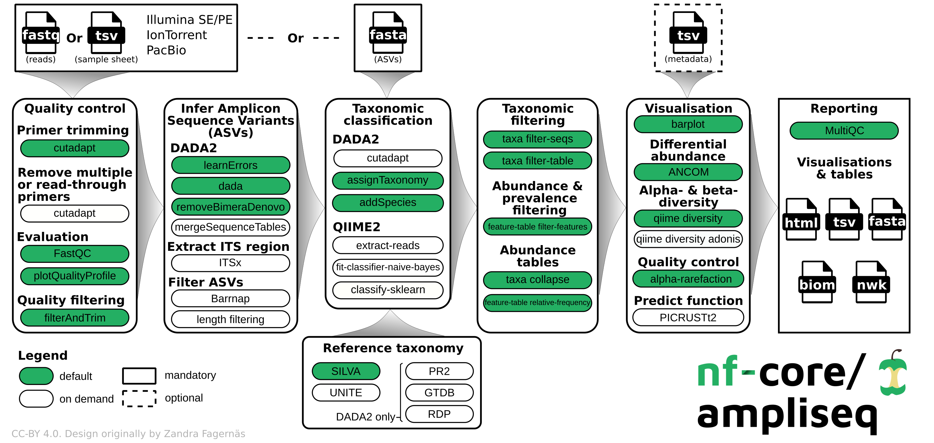
Microbial 16S (nf-core/ampliseq)

One of the most popular ways to measure the composition of microbial species in a complex mixture like the human microbiome is to amplify the 16S rRNA gene by PCR and perform high-throughput sequencing. By measuring the proportion of sequences which resemble a particular genus or species, one can estimate the proportion of the mixture of cells which was comprised by that taxon.

The nf-core/ampliseq pipeline uses two of the most popular software packages developed for this purpose: dada2 and QIIME2.

Supporting Media

User Guide

Inputs: The nf-core/ampliseq workflow can be run on two different types of inputs:

1. A collection of FASTQ files containing high-throughput sequencing data; or,
2. A single FASTA file containing one or more 16S sequences, representing consensus ASVs.

When analyzing FASTQ data, additional information on experimental design (primers, etc.) are required.

Primers: Protocols for 16S sequencing vary widely in the PCR primers which are used to amplify the 16S rRNA gene. In order to run your analysis effectively, you must specify both the forward and reverse primer sequences which were used.

Metadata: Any metadata which is applied to the 16S samples via Cirro (either by uploading a samplesheet.csv along with the FASTQ files, or by manually updating the sample metadata in the web browser) will be provided to the nf-core/ampliseq workflow in its expected metadata format.

By default, all of those columns of metadata will be used for comparative analysis of the samples in the dataset. To use a specific column (or columns), use the metadata_category parameter.

Extended Parameters: The nf-core/ampliseq pipeline provides extensive options for read trimming and downstream analysis. For an extended discussion of the use of those parameters refer to its online documentation.

Workflow Repository: github.com/nf-core/ampliseq

Citations:

• nf-core/ampliseq: Straub D, Blackwell N, Langarica-Fuentes A, Peltzer A, Nahnsen S, Kleindienst S. Interpretations of Environmental Microbial Community Studies Are Biased by the Selected 16S rRNA (Gene) Amplicon Sequencing Pipeline. Front Microbiol. 2020 Oct 23;11:550420. doi: 10.3389/fmicb.2020.550420. PMID: 33193131; PMCID: PMC7645116.
• dada2: Callahan BJ, McMurdie PJ, Rosen MJ, Han AW, Johnson AJ, Holmes SP. DADA2: High-resolution sample inference from Illumina amplicon data. Nat Methods. 2016 Jul;13(7):581-3. doi: 10.1038/nmeth.3869. Epub 2016 May 23. PMID: 27214047; PMCID: PMC4927377.
• QIIME2: Bolyen E, Rideout JR, Dillon MR, Bokulich NA, Abnet CC, Al-Ghalith GA, Alexander H, Alm EJ, Arumugam M, Asnicar F, Bai Y, Bisanz JE, Bittinger K, Brejnrod A, Brislawn CJ, Brown CT, Callahan BJ, Caraballo-Rodríguez AM, Chase J, Cope EK, Da Silva R, Diener C, Dorrestein PC, Douglas GM, Durall DM, Duvallet C, Edwardson CF, Ernst M, Estaki M, Fouquier J, Gauglitz JM, Gibbons SM, Gibson DL, Gonzalez A, Gorlick K, Guo J, Hillmann B, Holmes S, Holste H, Huttenhower C, Huttley GA, Janssen S, Jarmusch AK, Jiang L, Kaehler BD, Kang KB, Keefe CR, Keim P, Kelley ST, Knights D, Koester I, Kosciolek T, Kreps J, Langille MGI, Lee J, Ley R, Liu YX, Loftfield E, Lozupone C, Maher M, Marotz C, Martin BD, McDonald D, McIver LJ, Melnik AV, Metcalf JL, Morgan SC, Morton JT, Naimey AT, Navas-Molina JA, Nothias LF, Orchanian SB, Pearson T, Peoples SL, Petras D, Preuss ML, Pruesse E, Rasmussen LB, Rivers A, Robeson MS 2nd, Rosenthal P, Segata N, Shaffer M, Shiffer A, Sinha R, Song SJ, Spear JR, Swafford AD, Thompson LR, Torres PJ, Trinh P, Tripathi A, Turnbaugh PJ, Ul-Hasan S, van der Hooft JJJ, Vargas F, Vázquez-Baeza Y, Vogtmann E, von Hippel M, Walters W, Wan Y, Wang M, Warren J, Weber KC, Williamson CHD, Willis AD, Xu ZZ, Zaneveld JR, Zhang Y, Zhu Q, Knight R, Caporaso JG. Reproducible, interactive, scalable and extensible microbiome data science using QIIME 2. Nat Biotechnol. 2019 Aug;37(8):852-857. doi: 10.1038/s41587-019-0209-9. Erratum in: Nat Biotechnol. 2019 Sep;37(9):1091. PMID: 31341288; PMCID: PMC7015180.

---

PacBio HiFi 16S

In addition to short read sequencing on the Illumina platform, the PacBio platform can be used to generate long HiFi reads that cover a very large portion of the microbial 16S rRNA gene. These long sequences can be used to identify bacteria from complex mixtures with a much higher degree of taxonomic specificity than short read sequencing.

The analysis of PacBio HiFI 16S data is performed on Cirro using a workflow developed by PacBio which employs the industry-standard tools DADA2 and QIIME2.

Supports combining input datasets in a single analysis.

Parameters:

• Forward Primer Sequence (default: AGRGTTYGATYMTGGCTCAG)
• Reverse Primer Sequence (default: AAGTCGTAACAAGGTARCY)
• Filter Quality Threshold (Filter input reads above this Q value)
• Minimum Quality (Reads with any base lower than this quality score will be removed)
• Minimum Length (Sequences shorter than this will be discarded)
• Maximum Length (Sequences longer than this will be discarded)
• Maximum Expected Errors (Reads with number of expected errors higher than this value will be discarded)
• Pooling Method (QIIME 2 pooling method for DADA2 denoising)
• Max Reject (QIIME 2 max-reject parameter for VSEARCH taxonomy classification method)
• Max Accept (QIIME 2 max-accept parameter for VSEARCH taxonomy classification method)
• Minimum Identity (Minimum identity to be considered as hit)
• Minimum Counts per ASV (Total counts of any ASV across all samples must be above this threshold to be retained)
• Minimum Samples per ASV (Minimum number of samples that an ASV must be found in to be retained)

Workflow Repository: github.com/PacificBiosciences/HiFi-16S-workflow

---

Taxonomic Classification (MetaPhlAn4)

When performing high-throughput DNA sequencing there are many reasons why a researcher may want to identify the organisms present in the source sample. While this process of 'taxonomic classification' was originally developed for the purpose of microbiome analysis, it can also be helpful for identifying potential contaminants in putatively pure samples.

Because there are so many different algorithms for taxonomic classification of WGS datasets, the Critical Assessment of Metagenome Interpretation (CAMI) challenge was established to provide an unbiased estimate of the accuracy for those methods. One of the top-performing methods for taxonomic classification was MetaPhlAn (which also happens to be one of the original tools developed for this purpose).

Defining Inputs

Taxonomic classification may be performed using either paired-end or single-end FASTQ files. More than one set of FASTQ files may be provided for each sample, if needed. Sample names can be mapped to input files by including a samplesheet.csv file in the input directory. Note that the column names in the samplesheet.csv file must include sample, fastq_1, and fastq_2 (if paired-end reads are provided). Additional columns may be used to provide metadata for each sample.

Example samplesheet.csv:

sample,fastq_1,fastq_2,age
sample_A,sample_A_R1.fastq.gz,sample_A_R2.fastq.gz,30
sample_B,sample_B_R1.fastq.gz,sample_B_R2.fastq.gz,45
sample_C,sample_C1_R1.fastq.gz,sample_C1_R2.fastq.gz,25
sample_C,sample_C2_R1.fastq.gz,sample_C2_R2.fastq.gz,25

Supports combining input datasets in a single analysis.

Per-Sample Analysis

Each sample is analyzed independently, using either paired-end or single-end reads (as provided)

metaphlan \
    ${fastq_1},${fastq_2} \
    --input_type fastq \
    --bowtie2db ${db} \
    -t rel_ab_w_read_stats \
    --unclassified_estimation \
    --sample_id "${sample_name}"

Combined Abundance Tables

Microbial abundances generated for each sample are combined into a single set of abundance tables, which can be used for downstream analysis.

In addition to the merge_metaphlan_tables.py command provided by MetaPhlAn, summary tables are provided for each taxonomic level (species, genus, etc.).

Reference Database:

The reference database used for MetaPhlAn is periodically updated to include new organisms which have been added to the reference databases. The most recent database available is v30 (January 19, 2020), and any newer databases will be added to the portal as they become available.

More Details

Tool Documentation:

The biobakery group maintains an extremely useful collection of documentation for MetaPhlAn which may be helpful in understanding the operation and output of the tool.

Workflow Repository: github.com/FredHutch/metaphlan-nf

Citations:

• MetaPhlAn: Segata, N., Waldron, L., Ballarini, A. et al. Metagenomic microbial community profiling using unique clade-specific marker genes. Nat Methods 9, 811–814 (2012). https://doi.org/10.1038/nmeth.2066
• MetaPhlAn4: Extending and improving metagenomic taxonomic profiling with uncharacterized species with MetaPhlAn 4. Aitor Blanco-Miguez, Francesco Beghini, Fabio Cumbo, Lauren J. McIver, Kelsey N. Thompson, Moreno Zolfo, Paolo Manghi, Leonard Dubois, Kun D. Huang, Andrew Maltez Thomas, Gianmarco Piccinno, Elisa Piperni, Michal Punčochář, Mireia Valles-Colomer, Adrian Tett, Francesca Giordano, Richard Davies, Jonathan Wolf, Sarah E. Berry, Tim D. Spector, Eric A. Franzosa, Edoardo Pasolli, Francesco Asnicar, Curtis Huttenhower, Nicola Segata. bioRxiv 2022.08.22.504593; doi: https://doi.org/10.1101/2022.08.22.504593

---

Taxonomic Classification (Sourmash)

In addition to the marker-based approaches for taxonomic classification of WGS data, a widely adopted approach has been exact alignment against large whole-genome databases of short sequence fragments ("k-mers").

One computational analysis tool which has broad functionality and has performed well in a comparison across methods is sourmash. This analysis includes:

1. Aligning each WGS dataset against a pre-built k-mer database
2. Identifying the reference genomes with greatest nucleotide similarity
3. Summarizing the taxonomic composition of each sample

Supports combining input datasets in a single analysis.

Analysis Parameters:

• Database Size: Number of genomes contained in the reference database used to search against in the GTDB R08-RS214 database (85k or 403k)
• K-mer Length: Length (k) of strings used for exact-match search against the reference database (21bp, 31bp, or 51bp)
• Minimum Match Threshold: Minimum number of basepairs which must be found uniquely for a genome to be retained

Workflow Repository: github.com/CirroBio/nf-sourmash

Citations:

• Lightweight compositional analysis of metagenomes with FracMinHash and minimum metagenome covers Luiz Irber, Phillip T. Brooks, Taylor Reiter, N. Tessa Pierce-Ward, Mahmudur Rahman Hera, David Koslicki, C. Titus Brown bioRxiv 2022.01.11.475838; doi: https://doi.org/10.1101/2022.01.11.475838
• Pierce NT, Irber L, Reiter T et al. Large-scale sequence comparisons with sourmash [version 1; peer review: 2 approved]. F1000Research 2019, 8:1006 (https://doi.org/10.12688/f1000research.19675.1)

---

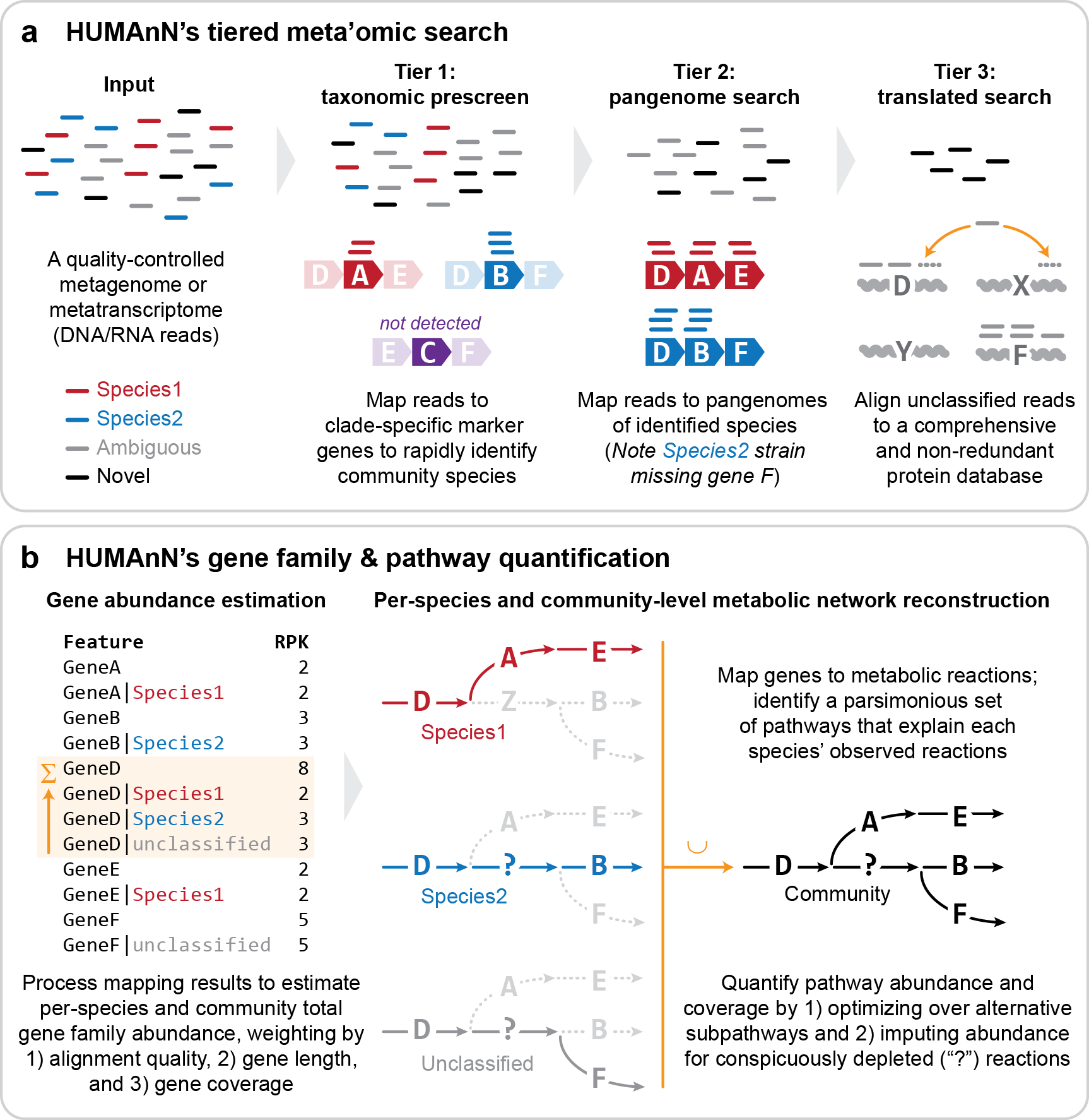
Metagenomic Pathways (HUMAnN)

HUMAnN (the HMP Unified Metabolic Analysis Network) is a method for efficiently and accurately profiling the abundance of microbial metabolic pathways and other molecular functions from metagenomic or metatranscriptomic sequencing data. It is appropriate for any type of microbial community, not just the human microbiome (the name "HUMAnN" is a historical product of the method's origins in the Human Microbiome Project). (Source: HUMAnN Documentation)

Supports combining input datasets in a single analysis.

Reference Databases:

HUMAnN offers four different reference databases which provide a trade-off of sensitivity in exchange for speed.

The UniRef90 databases contain gene families clustered at 90% amino acid identity, while UniRef50 provides a coarser level of 50% amino acid identity. More details on UniRef can be found on their website.

In addition to the full databases, it is also possible to search against a vastly smaller database which only contains gene families which have a level-4 enzyme commission (EC) category assigned. Because only a small fraction of bacterial genes have been annotated, these databases will not capture the bulk of microbial gene families.

The options available are:

• Full UniRef90 (20.7GB, recommended)
• EC-filtered UniRef90 (0.9GB)
• Full UniRef50 (6.9GB)
• EC-filtered UniRef50 (0.3GB)

Output Files:

Gene Families (humann_genefamilies.tsv)

The relative abundance (proportion) of reads assigned to each gene family are shown across all samples. Each gene family's total abundance is broken down into the contributions from individual organisms when possible (delineated by the pipe character: |). For example:

UniRef90_G1UL42|g__Bacteroides.s__Bacteroides_dorei

You can also learn more about a given UniRef family by looking up its representative protein on the UniProt website (note the removal of the UniRef90_ prefix): https://www.uniprot.org/uniprot/G1UL42

Pathway Abundances (humann_pathabundance.tsv)

The proportion of organisms encoding each metabolic pathway is summarized across all samples. For details on the calculation of pathway abundances from constituent gene family abundances, see the HUMAnN User Manual. Like gene families, pathways are broken down into per-organism contributions when possible (again delineated by the | character). (Source: HUMAnN Documentation)

Per-Sample Outputs

In addition to the merged tables described above, the outputs for each sample will be available in a set of folders named for the sample. This will include:

• SAMPLE_genefamilies.tsv - Depth of sequencing (reads-per-kilobase, RPK) for each gene family
• SAMPLE_genefamilies_relabund.tsv - Relative abundance of each gene family
• SAMPLE_pathabundance.tsv - Depth of sequencing (reads-per-kilobase, RPK) for each pathway
• SAMPLE_pathabundance_relabund.tsv - Relative abundance of each pathway
• SAMPLE_pathcoverage.tsv - Coverage (proportion of genes detected at all) for each pathway

Tool Documentation:

The biobakery group maintains an extremely useful collection of documentation for HUMAnN which may be helpful in understanding the operation and output of the tool.

Workflow Repository: github.com/CirroBio/nf-humann

Citations:

• Francesco Beghini, Lauren J McIver, Aitor Blanco-Míguez, Leonard Dubois, Francesco Asnicar, Sagun Maharjan, Ana Mailyan, Paolo Manghi, Matthias Scholz, Andrew Maltez Thomas, Mireia Valles-Colomer, George Weingart, Yancong Zhang, Moreno Zolfo, Curtis Huttenhower, Eric A Franzosa, Nicola Segata (2021) Integrating taxonomic, functional, and strain-level profiling of diverse microbial communities with bioBakery 3 eLife 10:e65088 https://doi.org/10.7554/eLife.65088

---

Microbial Genome Annotation (prokka / gapseq)

After determining the nucleotide sequence of a microbial genome, a researcher may want to inspect the genetic content in terms of the genes present and the metabolic pathways which are encoded. By marking the physical regions of the genomes which are predicted to contain different genes, a researcher can gain some understanding of its behavior and activities. The annotation files produced through this process can be inspected visually using a variety of different desktop applications, and may also be used to support their submission to sequence repositories.

User Guide

Genome Annotation - Prokka:

One of the most widely used software libraries for bacterial genome annotation is Prokka, maintained by Prof. Torsten Seemann. This utility combines the functions of multiple components, including:

• Prodigal to find protein-coding features (CDS)
• Aragorn to find transfer RNA features (tRNA)
• Barrnap to predict ribosomal RNA features (rRNA)
• HMMER3 for similarity searching against protein family profiles

The output files produced by Prokka include (source):

Extension	Description
.gff	This is the master annotation in GFF3 format, containing both sequences and annotations. It can be viewed directly in Artemis or IGV.
.gbk	This is a standard Genbank file derived from the master .gff. If the input to prokka was a multi-FASTA, then this will be a multi-Genbank, with one record for each sequence.
.fna	Nucleotide FASTA file of the input contig sequences.
.faa	Protein FASTA file of the translated CDS sequences.
.ffn	Nucleotide FASTA file of all the prediction transcripts (CDS, rRNA, tRNA, tmRNA, misc_RNA)
.sqn	An ASN1 format "Sequin" file for submission to Genbank. It needs to be edited to set the correct taxonomy, authors, related publication etc.
.fsa	Nucleotide FASTA file of the input contig sequences, used by "tbl2asn" to create the .sqn file. It is mostly the same as the .fna file, but with extra Sequin tags in the sequence description lines.
.tbl	Feature Table file, used by "tbl2asn" to create the .sqn file.
.err	Unacceptable annotations - the NCBI discrepancy report.
.log	Contains all the output that Prokka produced during its run. This is a record of what settings you used, even if the --quiet option was enabled.
.txt	Statistics relating to the annotated features found.
.tsv	Tab-separated file of all features: locus_tag,ftype,len_bp,gene,EC_number,COG,product

Metabolic Pathway Prediction - gapseq:

The in silico prediction of metabolic pathways from primary genomic sequence is an emerging field of study. While there are a handful of published methods, gapseq was selected for use in this analysis workflow on the basis of its robust deployment and execution.

The steps performed by gapseq include:

• prediction of metabolic pathways from various databases
• transporter inference
• metabolic model construction
• multi-step gap filling

Workflow Repository: github.com/FredHutch/prokka-nf

Citations:

• Prokka: Seemann T. Prokka: rapid prokaryotic genome annotation. Bioinformatics 2014 Jul 15;30(14):2068-9. PMID:24642063
• Prodigal: Hyatt D et al. Prodigal: prokaryotic gene recognition and translation initiation site identification. BMC Bioinformatics. 2010 Mar 8;11:119.
• Aragorn: Laslett D, Canback B. ARAGORN, a program to detect tRNA genes and tmRNA genes in nucleotide sequences. Nucleic Acids Res. 2004 Jan 2;32(1):11-6.
• HMMER3: Finn RD et al. HMMER web server: interactive sequence similarity searching. Nucleic Acids Res. 2011 Jul;39(Web Server issue):W29-37.
• gapseq: Zimmermann, J., Kaleta, C. & Waschina, S. gapseq: informed prediction of bacterial metabolic pathways and reconstruction of accurate metabolic models. Genome Biology 22, 81 (2021)

---

Microbial Pangenome Anvi'o

Because of the high degree of diversity within microbial genomes, the term "pangenome" is used to refer to the aggregate content of a collection of genomes. When inspecting a bacterial pangenome, it is very common to find that there are large groups of genes which are found in only a subset of genomes. These blocks of genomic content very often define clades or subspecies, but can also be associated with horizontal gene transfer.

The anvi'o pangenome analysis tool is used widely in the field to summarize the content of a collection of microbial genomes. This includes:

• Identifying gene clusters (similar genes across genomes)
• Estimating relationships of genomes based on gene clusters
• Annotating the likely function of amino acid sequences
• Identifying gene clusters or functions enriched in a subset of genomes

The anvi'o software suite also provides an interactive viewer which can be installed on your computer to provide a rich visualization interface using the output from the pangenome analysis tool.

Supports combining input datasets in a single analysis.

User Guide

Analysis Parameters:

• mcl_inflation: Gene Clustering Threshold (mcl_inflation)
  • Ranges from 2 (approximately species-level) to 10 (approximately strain-level)
  • default: 2
• minbit: Sequence Similarity Threshold (minbit)
  • Threshold of sequence similarity used to group genes (ranges 0-1)
  • default: 0.5
• min_occurrence: Minimum Occurrence
  • Filter out any genes which are found in fewer than this number of genomes
  • default: 1
• min_alignment_fraction: Minimum Alignment Fraction
  • Any pairwise genome ANI scores below this threshold will be set to zero
  • default: 0.0
• category_name: Compare Genomes By
  • Optional genome metadata attribute used to compare genomes
• gene_enrichment: Calculate Gene-Level Enrichment
  • Instead of using functional groupings, enrichment scores can be calculated on a per-gene basis
  • default: false
• distance: Distance Metric
  • Metric used to summarize genome similarity
  • default: euclidean
• linkage: Linkage Method
  • Method used to build tree of genomes
  • default: ward

Workflow Repository: github.com/FredHutch/nf-anvio-pangenome

Citations:

• Eren, A.M., Kiefl, E., Shaiber, A. et al. Community-led, integrated, reproducible multi-omics with anvi’o. Nat Microbiol 6, 3–6 (2021). https://doi.org/10.1038/s41564-020-00834-3

---

Microbial Pangenome (gig-map)

In addition to the anvi'o software suite, microbial pangenomes can be built using the gig-map bioinformatics workflow.

Analysis Steps:

• Deduplicate gene sequences with CD-HIT
• Identify which genomes contain each gene with DIAMOND or BLAST
• Bin genes together based on co-occurrence across genomes
• Group genomes together based on shared gene content

graph TD;
    Genomes --> align[Align Genes to Genomes];
    Genes --> deduplicate[Deduplicate Genes];
    deduplicate --> align;
    align --> filter_genes[Filter Genes by Frequency];
    filter_genes --> bin_genes[Bin Genes];
    bin_genes --> filter_bins[Filter Bins by Size]
    align --> cluster_genomes[Cluster Genomes];
    cluster_genomes --> summarize[Summarize];
    filter_bins --> summarize;

Supports combining input datasets in a single analysis.

Parameters:

• Minimum Coverage: Minimum proportion of a gene which must align in order to retain the alignment (default: 90)
• Minimum Percent Identity: Minimum percent identity of the amino acid alignment required to retain the alignment (default: 90)
• Maximum Overlap: Any alignment which overlaps a higher-scoring alignment by more than this amount will be filtered out (default: 50)
• Maximum E-Value: Maximum E-value threshold used to filter all alignments default (default: 0.001)
• Genetic Code: Translation table used for conceptual translation of nucleotides to protein default (default: 11)
• Aligner: Algorithm for aligning genes to genomes - DIAMOND (default) or BLAST
• Gene Clustering Threshold: Maximum Jaccard distance threshold used to group genes into bins (default: 0.05)
• Genome Clustering Threshold: Maximum Euclidean distance threshold used to group genomes based on gene bin content (default: 0.05)
• Minimum Bin Size: Minimum number of genes needed to retain a bin (default: 1)
• Minimum Gene Frequency: Minimum number of genomes for a gene to be found in to be included (default: 1)

Workflow Repository: github.com/FredHutch/gig-map

Citations:

• Sayers EW, Bolton EE, Brister JR, Canese K, Chan J, Comeau DC, Connor R, Funk K, Kelly C, Kim S, Madej T, Marchler-Bauer A, Lanczycki C, Lathrop S, Lu Z, Thibaud-Nissen F, Murphy T, Phan L, Skripchenko Y, Tse T, Wang J, Williams R, Trawick BW, Pruitt KD, Sherry ST. Database resources of the national center for biotechnology information. Nucleic Acids Res. 2022 Jan 7;50(D1):D20-D26. doi: 10.1093/nar/gkab1112. PMID: 34850941; PMCID: PMC8728269.
• Buchfink, B., Xie, C. & Huson, D. Fast and sensitive protein alignment using DIAMOND. Nat Methods 12, 59–60 (2015). https://doi.org/10.1038/nmeth.3176
• Fu L, Niu B, Zhu Z, Wu S, Li W. CD-HIT: accelerated for clustering the next-generation sequencing data. Bioinformatics. 2012 Dec 1;28(23):3150-2. doi: 10.1093/bioinformatics/bts565. Epub 2012 Oct 11. PMID: 23060610; PMCID: PMC3516142.

---

Microbial Metagenome Aligned to Pangenome (gig-map)

After building a microbial pangenome, it can be useful to quantify the relative abundance of each gene group within a collection of metagenome samples. This analysis approach can be useful for comparing the relative abundance of organisms between groups of samples, identified on the basis of their gene content.

Analysis Steps:

• Align metagenome reads to the pangenome using DIAMOND
• Deduplicate any multi-mapping reads with FAMLI
• Filter samples using a minimum number of reads and genes detected
• Summarize the sequencing depth for each gene bin
• Compare the relative abundance of gene bins between samples

graph TD;
    Metagenomes --> align[Align Metagenomes to Pangenome];
    catalog[Gene Catalog] --> align;
    align --> dedup[Deduplicate Aligments];
    dedup --> filter_samples[Filter Samples];
    bins[Gene Bins] --> summarize[Summarize Gene Bins];
    filter_samples --> summarize;
    Metadata --> compare[Compare Samples];
    summarize --> compare;

Supports combining input datasets in a single analysis.

Parameters:

• Minimum Alignment Score: Alignment bitscore threshold applied on a per-read level (default: 50)
• Minimum Percent Identity: Minimum percent identity of the amino acid alignment required to retain the alignment (default: 90)
• Maximum E-Value: Maximum E-value threshold used to filter all alignments default (default: 0.001)
• Minimum Number of Reads: Minimum number of aligned reads required to retain a sample
• Minimum Number of Genes: Minimum number of aligned genes required to retain a sample
• Category: Optional: Compare sample groups based on a metadata variable

Workflow Repository: github.com/FredHutch/gig-map

Citations:

• Buchfink, B., Xie, C. & Huson, D. Fast and sensitive protein alignment using DIAMOND. Nat Methods 12, 59–60 (2015). https://doi.org/10.1038/nmeth.3176
• Golob JL, Minot SS. In silico benchmarking of metagenomic tools for coding sequence detection reveals the limits of sensitivity and precision. BMC Bioinformatics. 2020 Oct 15;21(1):459. doi: 10.1186/s12859-020-03802-0. PMID: 33059593; PMCID: PMC7559173.

---

Curated Metagenomic Data

The Waldron Lab at the CUNY School of Public Health in New York City has produced curatedMetagenomicData a valuable resource for the microbiome community.

A large number of microbiome studies have been processed using the MetaPhlAn3 and HUMAnN3 analysis pipelines in a standardized way, which helps facilitate cross-study comparisons. Data is available for:

• relative_abundance (MetaPhlAn3)
• marker_presence (MetaPhlAn3)
• marker_abundance (MetaPhlAn3)
• gene_families (HUMAnN3)
• pathway_coverage (HUMAnN3)
• pathway_abundance (HUMAnN3)

Datasets output by the curatedMetagenomicDataTerminal are formatted in a particular way - with metadata columns concatenated with data columns in a single tab-delimited file. For this reason, a dedicated dataset type is available for sharing and analyzing information obtained from this community resource.

NOTE: The --counts flag is recommended when using the curatedMetagenomicDataTerminal tool to produce data for running Differential Abundance. When that flag is used, sequencing depth information is used to extrapolate the number of discrete genome fragments identified from each organism. This added information helps provide power for statistical modeling using the corncob algorithm.

Citation:

• Pasolli E, Schiffer L, Manghi P, Renson A, Obenchain V, Truong D, Beghini F, Malik F, Ramos M, Dowd J, Huttenhower C, Morgan M, Segata N, Waldron L (2017). “Accessible, curated metagenomic data through ExperimentHub.” Nat. Methods, 14(11), 1023–1024. ISSN 1548-7091, 1548-7105, doi:10.1038/nmeth.4468.

---

Microbial Abundance Table

Microbial abundance data is often made available directly in the form of a table containing either read count or proportional abundance measurements. Such datasets can be uploaded directly to Cirro along with sample metadata and used for downstream analysis such as differential abundance analysis.

The format expected for microbial abundance tables are:

• CSV format (using the .csv file extension)
• Each row is a sample, each column is a taxon
• Values may be integer counts or decimal proportions

Additional metadata may optionally be uploaded in a file named samplesheet.csv which similarly is formatted with each row as a sample and each column as a metadata field.

Useful tips:

• Downstream analysis in R (e.g. corncob) does not work well with sample names, organism names, or metadata categories that start with numbers or contain any non-alphanumeric values
• Binary metadata categories are best encoded as 0 vs. 1

---

Differential Abundance Analysis

One of the most common uses for microbiome data is to identify organisms which are present at higher or lower abundances between different groups of samples. This may be comparison across states of health and disease, or even biogeographical studies across space and time.

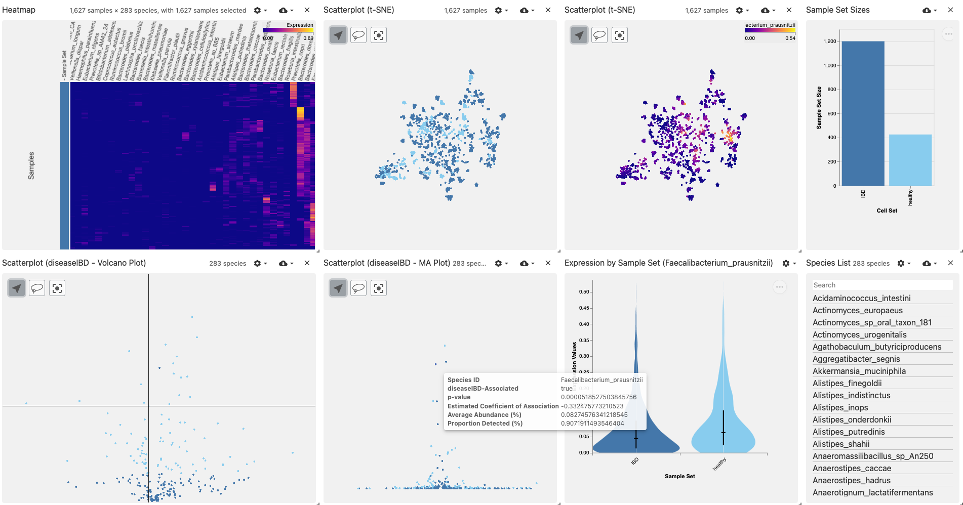
Results include:

• Summary of the top organisms detected across all samples
• Clustering of samples by taxonomic beta-diversity (t-SNE)
• Display of user-selected organism abundance across samples
• Volcano plot and MA plot showing the results of statistical analysis
• Comparison of the abundance of a user-selected organism between sample groups

The Differential Abundance pipeline provides a single analysis tool which can be used to analyze the relative abundance data produced by either 16S amplicon sequencing or WGS shotgun metagenomic sequencing (also called WMS).

Input datasets can be generated with either:

• nf-core/ampliseq (16S)
• MetaPhlAn (WGS)
• Sourmash (WGS)
• curatedMetagenomicData
• Microbial Abundance Tables

When uploading data, simply provide the sample metadata category to be used as the basis of comparison:

sample,fastq_1,fastq_2,study_group
sampleA,sampleA_R1.fastq.gz,sampleA_R2.fastq.gz,A
sampleB,sampleB_R1.fastq.gz,sampleB_R2.fastq.gz,A
sampleC,sampleC_R1.fastq.gz,sampleC_R2.fastq.gz,B
sampleD,sampleD_R1.fastq.gz,sampleD_R2.fastq.gz,B

And then use that sample metadata (e.g. study_group) to run the differential abundance analysis.

Supports combining input datasets in a single analysis.

Statistical Analysis:

The preferred analysis method used for differential abundance analysis is corncob, which performs count regression for correlated observations using the beta-binomial. It is possible to run analyses for one variable or a combination of variables using multivariate expressions (like "colA + colB").

For datasets with very low numbers of samples, the more general Mann Whitney U test is provided as an option for analysis.

Parameters:

• Formula: Metadata column(s) used for statistical analysis (e.g. "study_group")
• Statistical Method: Analysis tool used to compare the relative abundance between groups (default: corncob)
• FDR Cutoff: FDR-adjusted p-value threshold used to annotate significant results (default: 0.05)
• Minimum Abundance Display Threshold: (default: Only display organisms which meet this minimum proportion threshold in at least one sample)

Workflow Repository: github.com/CirroBio/nf-differential-abundance

Citations:

• corncob: Bryan D. Martin, Daniela Witten, and Amy D. Willis. (2020). Modeling microbial abundances and dysbiosis with beta-binomial regression. Annals of Applied Statistics, Volume 14, Number 1, pages 94-115.